The last decade of AI research has been characterised by the exploration of the potential of deep neural networks. The advances we have seen in recent years can be at least partly attributed to the increasing size of networks. Considerable effort has been put into creating larger and more complex architectures capable of increasingly impressive feats, from text generation with GPT-3 [1] to image generation with Imagen [2]. Moreover, the success of modern neural networks has led to their deployment in a wide variety of applications. Even as I'm writing this, a neural network is attempting to predict the next word I'm about to write, albeit not accurately enough to replace me anytime soon!
Performance optimisation, on the other hand, has received relatively little attention in the field, which is a significant obstacle to the wider deployment of neural networks. A likely reason for this is the ability to train large neural networks in data centres on thousands of GPUs or other hardware simultaneously. This contrasts with the field of computer graphics for example, where the constraint of having to run in real-time on a single computer created a strong incentive to optimise algorithms without sacrificing quality.
Research in neural network capacity suggests that network capacities needed to discover high-accuracy solutions are greater than capacities needed to represent these solutions. In their paper, The Lottery Ticket Hypothesis: Finding Sparse, Trainable Neural Networks, Frankle and Carbin [3] found that only a small fraction of weights in a network are needed to represent a good solution, but directly training a reduced capacity network doesn’t lead to the same level of accuracy. Similarly, Hinton et al. [4] found that transferring “knowledge” from a high-accuracy network to a low-capacity one can produce a network with higher accuracy than training using the same loss function as the high-capacity network.
In this blog post, we ask whether it is possible to dynamically reduce a network’s parameters while training. While doing this is challenging, due to implementation complexity (PyTorch wasn’t designed to handle dynamic network architectures, e.g., the removal of entire channels during training), we expect to achieve the following advantages.
- Reduced number of weights in the final network.
- Reduced bit-depth of the remaining weights.
- Reduced runtime of the final network.
- Reduced training time.
- Reduced complexity in choosing layer widths when designing a network architecture.
- No special hardware is needed to take advantage of most optimisations (e.g., no need for sparse matrix multiplication).
In this work, we achieve these goals by introducing a novel quantisation-aware training (QAT) scheme that balances the requirements for maximising network accuracy and minimizing network size. We simultaneously maximise accuracy and minimise weight bit-depths, leading to the elimination of less important or unnecessary channels, thereby reducing compute and bandwidth requirements in a way that can be exploited easily by existing hardware.
Differentiable Quantisation
This is achieved through differentiable quantisation, as introduced in my previous post [5]. In short, differentiable quantisation allows you to learn the parameters of the number format simultaneously with the weights. This allows quantisation to be learned in exactly the same way as the weights in the network and enables new technologies such as self-compressing networks – the subject of this post.
The quantisation function used here quantises to a variable bit rate signed fixed point format:

This can be described as the sequence of the following steps.
- Scale the input value using the exponent:

- Clamp the value using the bit depth:

- Round to the nearest integer:

- Reverse the scaling introduced in step 1:

Where  is the bit depth,
  is the exponent and
  is the value (or set of values) being quantised. To ensure continuous differentiability, we use a real-valued bit-depth parameter during training.
The above function uses a rounding operation. The usual way of propagating a usable gradient back through this is to define the gradient of the rounding operation as 1 instead of 0. This is similar to the “straight-through estimator” [6]. To see why this works, consider the following figure:
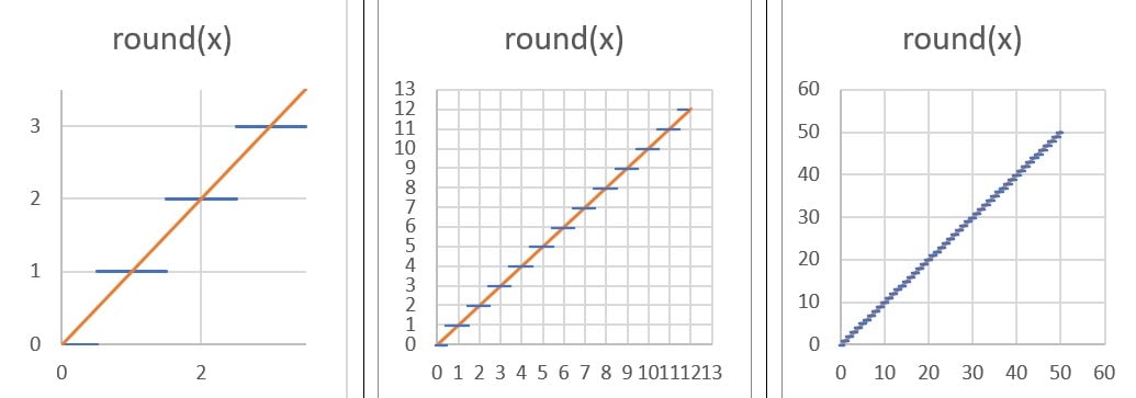
You can see how, as we “zoom out” from the function; the rounding function appears to approach the line y=x. We exploit this by replacing the backward pass (the gradient) of the rounding function with the gradient of the function y=x, i.e., a constant 1.
Self-compression through differentiable quantisation
In this work, we use differentiable quantisation (1) to reduce the bit depths of the network’s parameters during training (i.e., to compress it), and (2) to discover which parameters can be represented with 0 bits. A parameter in a neural network is unnecessary when it can be represented by 0 bits without impacting the network's accuracy. When a channel in a weight tensor is discovered that can be represented with 0 bits, it is removed from the network during training. A side-effect of this is that training accelerates with time (see Figure 2). The process can be described as follows.
- Splitting the network's parameters into channels.
- Quantising each channel with a single quantisation parameter pair of bit depth and exponent .
- Train the network for its original task while simultaneously minimising all bit-depth parameters.
- When a bit-depth parameter reaches 0, remove the channel of network weights that the parameter encodes from the network. Since an entire output channel is eliminated, this reduces the size of the corresponding convolution and any subsequent ops that consume the output tensor, without changing the network output.
By removing empty (i.e., 0-bit) channels from the network during training we can accelerate training significantly without changing the training outcome: the training results in the same network that we would get if we only removed empty channels at the end.
Although the method described in this blog post learns to compress and eliminate channels, it is generalisable to other hardware-exploitable learned sparsity patterns.
Network architecture
The network architecture chosen was David Page's DAWNbench entry for CIFAR-10 [7] which is a shallow ResNet that can be trained quickly. Using a fast-training network has several advantages, including:
- makes algorithm design iteration faster,
- shortens the debug cycle,
- making it easy to perform experiments in a reasonable time on a single GPU,
- aiding reproduction of the results in this work.
This network consists of two main types of blocks: convolutional blocks (convolution → batch norm → activation → pooling) and residual blocks (with the residual branch consisting of two convolutional blocks). The following sections describe how to apply differentiable quantisation to these modules to make them compressible.
Optimisation objective
The goal of this work is to reduce the inference and training time of neural networks. To achieve this, a suitable proxy of inference time should be included in the loss function, so that minimising it results in a faster network. The proxy used in this case was network size, defined as the total number of bits used to represent the weights in the network. Activation tensor sizes or the number of ops required to compute the output of the layer could also be minimised as a proxy to network performance.
The size of a single weight tensor can be expressed using the product of the four tensor dimensions: output channels, input channels, filter height, and filter width (0, I, H, W). Since we quantise each output channel with a separate number format with a learnable number of bits for layer , the total number of bits used to represent the tensor is given by:
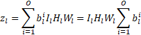
When  is 0 the
  th channel becomes unnecessary, reducing the total number of output channels in the weight tensor, and the corresponding input channels in the next convolution’s weight tensor. Therefore minimising
  makes it possible to minimise the number of elements in a weight tensor by minimising the number of output channels. This effectively minimises a weight tensor’s output dimension.
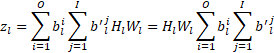
It’s possible to make the compression loss better reflect the size of the network by recognising that the number of input channels to a layer is equal to the number of output channels from the previous layer. This way a weight tensor’s input dimension can also be minimised:
Once a channel can be compressed to 0 bits it becomes a candidate for removal, possibly during training. However, a practical problem to overcome is that removing an output channel from a convolution layer doesn’t necessarily mean that the corresponding input channel can be removed safely from the next layer’s inputs since a bias could be added to a layer’s output of 0, in which case removing it might significantly change the network’s output. To handle this problem weight channels (filters) that reached 0 bits are identified and their outputs have an L1 loss applied to push them to 0 bits. Only when the biases were reduced to 0 are these filters removed, since at this point removing such a channel doesn’t change the network’s output.
The size of the entire network is the sum of the sizes of all layers:

To balance the accuracy and size of the network we simply use a linear combination of two terms:
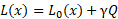
Where  is the original loss of the network, and
 ![]() is the compression factor. A larger
is the compression factor. A larger ![]() produces a smaller but less accurate network.
produces a smaller but less accurate network.
Handling branches
Another problem that arises when compressing a network is the handling of network branches, e.g., in residual blocks. The simplest solution to this problem is to consider the two branches separately.
Updating the optimiser
An implementation detail involves the problem of keeping the optimiser updated with the changes to the network. The optimiser tracks information (meta-parameters) about every parameter in the network, and when network parameters are dynamically removed, the corresponding meta-parameters must be removed from the optimiser as well.
Results
Self-compressing networks allow a trade-off between size and accuracy which can be visualised in a size-accuracy plot (see Figure 1). Each point in such a plot represents the size and accuracy of a neural network trained with a random compression rate , which is sampled from a log-uniform distribution covering the range  .
.
Figure 1 shows the relationship between the number of bits used to represent network weights compared to a 32-bit per weight baseline (corresponding to 32-bit floating point) when a network is trained with a random compression rate. This is computed as the percentage of weights kept, multiplied by the average bit depth of the remaining weights. The baseline accuracy of the network (the accuracy without compression) is 95.69 ± 0.22.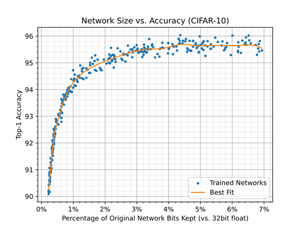
Figure 1: The relationship between the number of bits used to represent network weights compared to a 32-bit per weight baseline when a network is trained with a random compression rate.
Figure 2 shows only the reduction in the number of weights used in the network. Approximately 75% of the weights could be removed without impacting accuracy.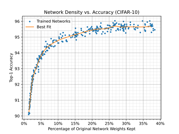
Figure 2 shows the relationship between the percentage of weights kept in the network and accuracy when a network is trained with a random compression rate.
Figure 3 shows the effect on training time by removing weights during training. The time to train for an epoch depends not only on the size of the network but also on other parts of the system, such as the input data pipeline. To determine a baseline training overhead, the same network was trained with only a single channel in each layer. This took approximately 7.5 seconds per epoch.
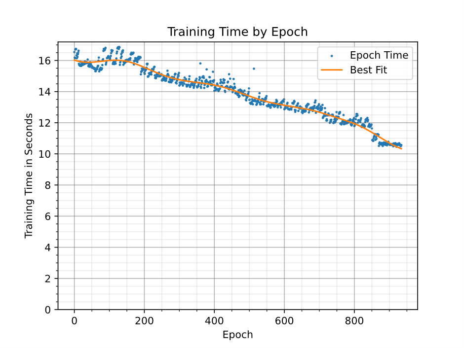
Figure 3: Neural network training time accelerates as parameters are removed from the network. 86% of weights were removed by the end of training.
Figure 4 shows the architecture of a network trained with a compression rate of  . The training removes the shortcut branch in the residual layer. The nine remaining channels already reached 0 bits by the end of training and were in the process of having their biases removed. They would be expected to disappear with longer training. The shortcut branch in the second residual layer had a very low loss associated with it (due to it contributing minimally to network size), so it was being reduced too slowly to disappear by the end of training.
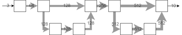
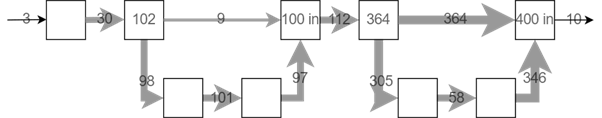
Figure 4: An example of layer sizes before and after training and average per-layer bit depths. Here 86% of weights and 97.6% of bits were removed. Each square represents a convolution. A value in a square represents the total number of output or input (“in”) channels of the convolution where such information is necessary (at branches).
Figure 5 shows the network size over the entire training process. It shrinks quickly early on and reduces more gradually later.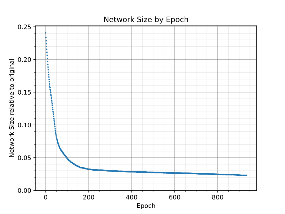
Figure 5: Network size shrinks fast early in training and reduces gradually later on.
Optimising your networks
In this blog post, we have shared a general framework for optimising typically fixed characteristics of neural networks -- the number of channels and bit depths – in such a way that the network learns to compress itself during training. The main advantages of this are faster execution time and training of the resulting network. Much of previous work focused on reducing network size by creating sparse layers, which needed special support in software and/or hardware to run more efficiently. Simply reducing the widths of layers doesn’t require specialised support. Supporting variable bit depths can increase performance on a wide range of architectures by reducing DRAM bandwidth.
References
|
[1] |
T. B. Brown and al, “Language Models are Few-Shot Learners,” 2020. |
|
[2] |
C. Saharia and al, “Photorealistic Text-to-Image Diffusion Models with Deep Language Understanding,” 2022. |
|
[3] |
J. Frankle and M. Carbin, “The Lottery Ticket Hypothesis: Finding Sparse, Trainable Neural Networks,” 2018. |
|
[4] |
G. Hinton, O. Vinyals and J. Dean, “Distilling the Knowledge in a Neural Network,” 2015. |
|
[5] |
Cséfalvay, S, “High-Fidelity Conversion of Floating-Point Networks for Low-Precision Inference using Distillation,” 25 May 2021. [Online]. Available: https://blog.imaginationtech.com/low-precision-inference-using-distillation/. |
|
[6] |
G. Hinton, “Lecture 9.3 — Using noise as a regularizer [Neural Networks for Machine Learning],” 2012. [Online]. Available: https://www.youtube.com/watch?v=LN0xtUuJsEI&list=PLoRl3Ht4JOcdU872GhiYWf6jwrk_SNhz9. |
|
[7] |
Page, D, “How to Train Your ResNet 8: Bag of Tricks,” 19 Aug 2019. [Online]. Available: https://myrtle.ai/how-to-train-your-resnet-8-bag-of-tricks/. |